Numerical continuation and bifurcation
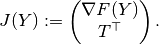
Let an algebraic problem coming from discretisation of a FEM-model can be written in the form

In what follows, we shall suppose that the model depends on an additional scalar
parameter  so that
 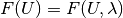 .
.
Numerical continuation
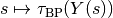
Methods of numerical continuation serve for tracing solutions of the system

In GetFEM++, a continuation technique for piecewise  (
( )
solution curves is implemented (see [Li-Re2014] for more details). Since it
does not make an explicit difference between the state variable
)
solution curves is implemented (see [Li-Re2014] for more details). Since it
does not make an explicit difference between the state variable  and
the parameter , we shall denote
and
the parameter , we shall denote  for
brevity. Nevertheless, to avoid bad scaling when calculating tangents, for
example, we shall use the following weighted scalar product and norm:
for
brevity. Nevertheless, to avoid bad scaling when calculating tangents, for
example, we shall use the following weighted scalar product and norm:

Here,  should be chosen so that
 is proportional to the scalar
product of the corresponding space variables, usually in
is proportional to the scalar
product of the corresponding space variables, usually in  . One can
take, for example,
. One can
take, for example,  , where
  is the mesh size and
 stands for the dimension of the underlying problem. Alternatively,
can be chosen as
stands for the dimension of the underlying problem. Alternatively,
can be chosen as  for simplicity.
The idea of the continuation strategy is to continue smooth pieces of solution curves by a classical predictor-corrector method and to join the smooth pieces continuously.
The particular predictor-corrector method employed is a slight modification of
the inexact Moore-Penrose continuation implemented in MATCONT [Dh-Go-Ku2003].
It computes a sequence of consecutive points  lying approximately
on a solution curve and a sequence of the corresponding unit tangent vectors
lying approximately
on a solution curve and a sequence of the corresponding unit tangent vectors
 :
:

To describe it, let us suppose that we have a couple  satisfying the relations above at our disposal. In the prediction, an initial
approximation of
satisfying the relations above at our disposal. In the prediction, an initial
approximation of  is taken as

where  is a step size. Its choice will be discussed later on.
In the correction, one computes a sequence
 , where
 and the couple
  is given by one
iteration of the Newton method applied to the equation
is given by one
iteration of the Newton method applied to the equation  with
with
and the initial approximation  . Due to the
potential non-differentiability of
. Due to the
potential non-differentiability of  , a piecewise-smooth variant of the
Newton method is used (Algorithm 7.2.14 in [Fa-Pa2003]).
, a piecewise-smooth variant of the
Newton method is used (Algorithm 7.2.14 in [Fa-Pa2003]).
Correction.
A couple  is accepted for
if
is accepted for
if
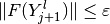 ,
,
 , and the
cosine of the angle between
, and the
cosine of the angle between  and is greater or
equal to
and is greater or
equal to  . Let us note that the partial gradient of
(or of one of its selection functions in the case of the
non-differentiability) with respect to is assembled analytically
whereas the partial gradient with respect to is evaluated by
forward finite differences with an increment equal to 1e-8.
. Let us note that the partial gradient of
(or of one of its selection functions in the case of the
non-differentiability) with respect to is assembled analytically
whereas the partial gradient with respect to is evaluated by
forward finite differences with an increment equal to 1e-8.
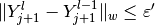
The step size  in the next prediction depends on how the Newton
correction has been successful. Denoting the number of iterations needed by
in the next prediction depends on how the Newton
correction has been successful. Denoting the number of iterations needed by
 , it is selected as
where  ,
,
 and
and
 are given constants. At the
beginning, one sets
are given constants. At the
beginning, one sets  for some
 .
.
Now, let us suppose that we have approximated a piece of a solution curve
corresponding to one sub-domain of smooth behaviour of and we want to
recover a piece corresponding to another sub-domain of smooth behaviour. Let
 be the last computed couple.
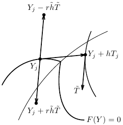
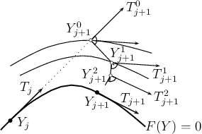
Transition between smooth pieces of a solution curve.
To approximate the tangent to the other smooth piece, we first take a point
 with a bit greater than
 so that this point belongs to the interior of the other
sub-domain of smooth behaviour. Then we find
so that this point belongs to the interior of the other
sub-domain of smooth behaviour. Then we find  such that

and it remains to determine an appropriate direction of this vector. This can be
done on the basis of the following observations: First, there exists
 such that
  remains
in the same sub-domain as for any
remains
in the same sub-domain as for any  positive.
This is characterised by the fact that
positive.
This is characterised by the fact that
 is significantly smaller than 1 for
  with
with
 . Second,
 appears in the other sub-domain for
larger than some positive threshold, and, for such values,
appears in the other sub-domain for
larger than some positive threshold, and, for such values,
 is close to 1 for
  with
with
 .
.
This suggests the following procedure for selecting the desired direction of
: Increase the values of successively from
, and when you arrive at and
such that
take  as the approximation of the tangent to the other smooth
piece.
as the approximation of the tangent to the other smooth
piece.
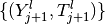
Having this approximation at our disposal, we restart the predictor-corrector
with  .
.
In GetFEM++, the continuation is implemented for two ways of parametrisation of the model:
The parameter
is directly a scalar datum, which the model
depends on.The model is parametrised by the scalar parameter
via a
vector datum  , which the model depends on. In this case, one takes
the linear path
, which the model depends on. In this case, one takes
the linear path
where
 and
and  are given values of , and one
traces the solution set of the problem
are given values of , and one
traces the solution set of the problem
Detection of limit points
When tracing solutions of the system  , one may be
interested in limit points (also called fold or turning points), where the
number of solutions with the same value of changes. These points
can be detected by a sign change of a test function
, one may be
interested in limit points (also called fold or turning points), where the
number of solutions with the same value of changes. These points
can be detected by a sign change of a test function  :
:
where is defined by

Limit point.
Numerical bifurcation
A point  is called a bifurcation point of the system
 if
if  and two or more distinct solution
curves pass through it. The following result gives a test for smooth
bifurcation points (see, e.g., [Georg2001]):
and two or more distinct solution
curves pass through it. The following result gives a test for smooth
bifurcation points (see, e.g., [Georg2001]):
Let  be a parametrisation of a solution curve and
 be a bifurcation point. Moreover, let
 ,
,
 ,
,
 ,
,  and
and
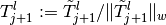
Define  via
via
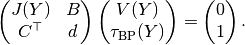
Then  changes its sign at
  .
.
Obviously, if one takes  ,
,  and randomly, it is
highly possible that they satisfy the requirements above. Consequently, the
numerical continuation method is able to detect bifurcation points by
taking the vectors
and randomly, it is
highly possible that they satisfy the requirements above. Consequently, the
numerical continuation method is able to detect bifurcation points by
taking the vectors  and
and  supplied by the correction at each
continuation step and monitoring the signs of
supplied by the correction at each
continuation step and monitoring the signs of  .
.
Once a bifurcation point is detected by a sign change
 , it can be
approximated more precisely by the predictor-corrector steps described above
with a special step-length adaptation (see Section 8.1 in [Al-Ge1997]). Namely,
one can take the subsequent step lengths as
, it can be
approximated more precisely by the predictor-corrector steps described above
with a special step-length adaptation (see Section 8.1 in [Al-Ge1997]). Namely,
one can take the subsequent step lengths as
until  , which corresponds to the
secant method for finding a zero of the function
, which corresponds to the
secant method for finding a zero of the function
 .
.
Finally, it would be desirable to switch solution branches. To this end, we shall consider the case of the so-called simple bifurcation point, where only two distinct solution curves intersect.
Let  be an approximation of that we are given
and
be an approximation of that we are given
and  be the first part of the solution of the augmented
system for computing the test function
be the first part of the solution of the augmented
system for computing the test function  . As
proposed in [Georg2001], one can take as a predictor
direction and do one continuation step starting with
. As
proposed in [Georg2001], one can take as a predictor
direction and do one continuation step starting with
 to obtain a point on a new branch. After this
continuation step has been performed successfully and a point on the new branch
has been recovered, one can proceed with usual predictor-corrector steps to
trace this branch.
to obtain a point on a new branch. After this
continuation step has been performed successfully and a point on the new branch
has been recovered, one can proceed with usual predictor-corrector steps to
trace this branch.
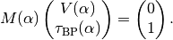
Recently, tools for numerical -bifurcation have been developed in
GetFEM++. Let  be a matrix function of a real parameter now defined by
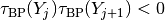
As proposed in [Li-Re2014hal], the following test can be used for detection of
a bifurcation point between and  :
:
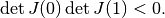
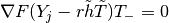
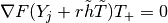
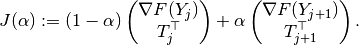
To perform this test numerically, introduce
and  analogously as above via
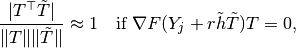
It follows from Cramer’s rule that
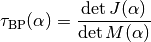
provided that  is non-zero. Hence if ,
and are chosen so that is non-zero whenever
is non-zero. Hence if ,
and are chosen so that is non-zero whenever
 is zero, then the sign changes of
are characterised by passings of through 0
whereas the sign changes of by sign changes of
caused by singularities. To conclude, the
sign of
is zero, then the sign changes of
are characterised by passings of through 0
whereas the sign changes of by sign changes of
caused by singularities. To conclude, the
sign of 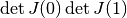 is determined by following the
behaviour of and monitoring the sign changes
of when
is determined by following the
behaviour of and monitoring the sign changes
of when  passes through
 ![[0,1]](../_images/math/e861e10e1c19918756b9c8b7717684593c63aeb8.png) .
.
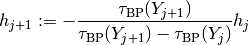
As justified in [Li-Re2014hal], , and can be
chosen randomly again. The increments  of the current values of
are changed adaptively so that singularities of
are treated effectively. After each calculation of
, is set as follows:
of the current values of
are changed adaptively so that singularities of
are treated effectively. After each calculation of
, is set as follows:
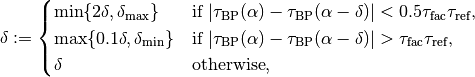
where 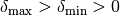 and
and
 are given constants and
 .
.
When a bifurcation point is detected between and
, it is approximated more precisely by a bisection-like
procedure. The obtained approximation lies on the same smooth branch as
 and the corresponding unit tangent that points out from the
corresponding region of smoothness is calculated too.
and the corresponding unit tangent that points out from the
corresponding region of smoothness is calculated too.
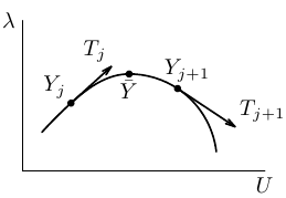
Contrary to the smooth case, it is not clear how many branches can emanate from
the bifurcation point and in which directions they could be
sought. For this reason, continuation steps for a whole sequence of predictor
directions are tried out for finding points on new branches.
Denoting , the approximation of the
bifurcation point and the corresponding tangent, respectively, the predictor
directions are taken as follows: For a couple of reference vectors
 and
and  , one takes
  with
with
 satisfying

where  passes through a set of linear combinations of
and . The total number of the linear
combinations is given by
passes through a set of linear combinations of
and . The total number of the linear
combinations is given by  and the reference vectors are
chosen successively according to the following strategy:
and the reference vectors are
chosen successively according to the following strategy:
One takes
 and such
that
and such
that
Let
 denote the
set of unit tangents that correspond to the points from the branches found so
far and that are oriented in the directions of branching from the bifurcation
point. Then and are taken
successively as different combinations from
.
denote the
set of unit tangents that correspond to the points from the branches found so
far and that are oriented in the directions of branching from the bifurcation
point. Then and are taken
successively as different combinations from
.If all combinations that are available so far have already been used, let
be unchanged and take
 with
with  satisfying
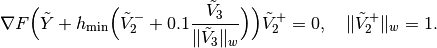
Here,
 equals the vector
employed previously and
equals the vector
employed previously and  is chosen randomly.
The total number of selections of and
is given by  .
.
More details on  numerical branching can be found in
[Li-Re2015hal].
numerical branching can be found in
[Li-Re2015hal].
Approximation of solution curves of a model
The numerical continuation is defined in getfem/getfem_continuation.h. In order to use it, one has to set it up via the corresponding object first:
getfem::cont_struct_getfem_model S(model, parameter_name, sfac, ls, h_init, h_max, h_min, h_inc, h_dec,
                                   maxit, thrit, maxres, maxdiff, mincos, maxres_solve, noisy, singularities,
                                   non-smooth, delta_max, delta_min, thrvar, ndir, nspan);
where parameter_name is the name of the model datum representing
, sfac represents the scale factor , and ls
is the name of the solver to be used for the linear systems incorporated in the
process (e.g., getfem::default_linear_solver<getfem::model_real_sparse_matrix, getfem::model_real_plain_vector>(model)). The real numbers h_init,
h_max, h_min, h_inc, h_dec denote  ,
,
 , ,
, ,  ,
and
,
and  , the integer maxit is the maximum number of
iterations allowed in the correction and thrit, maxres, maxdiff,
mincos, and maxres_solve denote
, the integer maxit is the maximum number of
iterations allowed in the correction and thrit, maxres, maxdiff,
mincos, and maxres_solve denote  ,
,
 ,
,  , , and the
target residual value for the linear systems to be solved, respectively. The
non-negative integer noisy determines how detailed information has to be
displayed in the course of the continuation process (the larger value the more
details), the integer singularities determines whether the tools for
detection and treatment of singular points have to be used (0 for ignoring them
completely, 1 for detecting limit points, and 2 for detecting and treating
bifurcation points, as well), and the boolean value of non-smooth determines
whether only tools for smooth continuation and bifurcation have to be used
or even tools for non-smooth ones do. The real numbers delta_max,
delta_min and thrvar represent
, , and the
target residual value for the linear systems to be solved, respectively. The
non-negative integer noisy determines how detailed information has to be
displayed in the course of the continuation process (the larger value the more
details), the integer singularities determines whether the tools for
detection and treatment of singular points have to be used (0 for ignoring them
completely, 1 for detecting limit points, and 2 for detecting and treating
bifurcation points, as well), and the boolean value of non-smooth determines
whether only tools for smooth continuation and bifurcation have to be used
or even tools for non-smooth ones do. The real numbers delta_max,
delta_min and thrvar represent  ,
,
 and
and  , and the integers
ndir and nspan stand for
, and the integers
ndir and nspan stand for  and
, respectively.
and
, respectively.
Optionally, parametrisation by a vector datum is then declared by:
S.set_parametrised_data_names(initdata_name, finaldata_name, currentdata_name);
Here, the data names initdata_name and finaldata_name should represent
and , respectively. Under currentdata_name, the
values of  have to be stored, that is, actual values of the
datum the model depends on.
have to be stored, that is, actual values of the
datum the model depends on.
Next, the continuation is initialised by:
S.init_Moore_Penrose_continuation(U, lambda, T_U, T_lambda, h);
where U should be a solution for the value of the parameter
equal to lambda so that  (U,lambda). During
this initialisation, an initial unit tangent
(U,lambda). During
this initialisation, an initial unit tangent  corresponding to
 is computed in accordance with the sign of the initial value
T_lambda, and it is returned in T_U, T_lambda. Moreover, h is
set to the initial step size h_init.
is computed in accordance with the sign of the initial value
T_lambda, and it is returned in T_U, T_lambda. Moreover, h is
set to the initial step size h_init.
Subsequently, one step of the continuation is called by
S.Moore_Penrose_continuation(U, lambda, T_U, T_lambda, h, h0);
After each call, a new point on a solution curve and the corresponding tangent are returned in the variables U, lambda and T_U, T_lambda. The step size for the next prediction is returned in h. The size of the current step is returned in the optional argument h0. According to the chosen value of singularities, the test functions for limit and bifurcation points are evaluated at the end of each continuation step. Furthermore, if a smooth bifurcation point is detected, the procedure for numerical bifurcation is performed and an approximation of the branching point as well as tangents to both bifurcating curves are saved in the continuation object S. From there, they can easily be recovered with member functions of S so that one can initialise the continuation to trace either of the curves next time.
Complete examples of use on a smooth problem are shown in the test programs tests/test_continuation.cc, interface/tests/matlab/demo_continuation.m and interface/src/scilab/demos/demo_continuation.sce, whereas interface/src/scilab/demos/demo_continuation_vee.sce and interface/src/scilab/demos/demo_continuation_block.sce employ also non-smooth tools.
![]()
Table Of Contents
Previous topic
Large sliding/large deformation contact with friction bricks
Next topic
Finite strain Elasticity bricks
Download
Main documentations
- GetFEM++ User documentation
- Python Interface
- Matlab Interface
- Scilab Interface
- Gmm++
- GetFEM++ project