Appendix A. Finite element method list
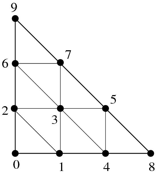
Symbols representing degree of freedom types 

Value of the function at the node. Value of the gradient along of the first coordinate. Value of the gradient along of the second coordinate. 
Value of the gradient along of the thrid coordinate for 3D elements. Value of the whole gradient at the node. Value of the normal derivative to a face. 
Value of the second derivative along the first coordinate (twice). Value of the second derivative along the second coordinate (twice). Value of the second cross derivative in 2D or second derivative along the thrid coordinate (twice) in 3D. 
Value of the whole second derivative (hessian) at the node. Scalar product with a certain vector (for instance an edge) for a vector elements. Scalar product with the normal to a face for a vector elements. 

Bubble function on an element or a face, to be specified. Lagrange hierarchical d.o.f. value at the node in a space of details.
Let us recall that all finite element methods defined in GetFEM++ are declared in the file getfem_fem.h and that a descriptor on a finite element method is obtained thanks to the function:
getfem::pfem pf = getfem::fem_descriptor("name of method");
where "name of method" is a string to be choosen among the existing methods.
Classical  Lagrange elements on simplices
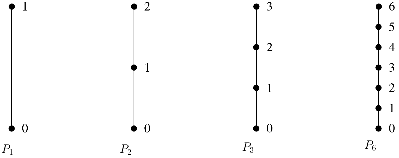
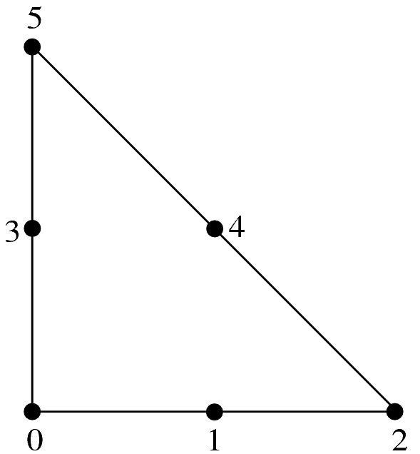
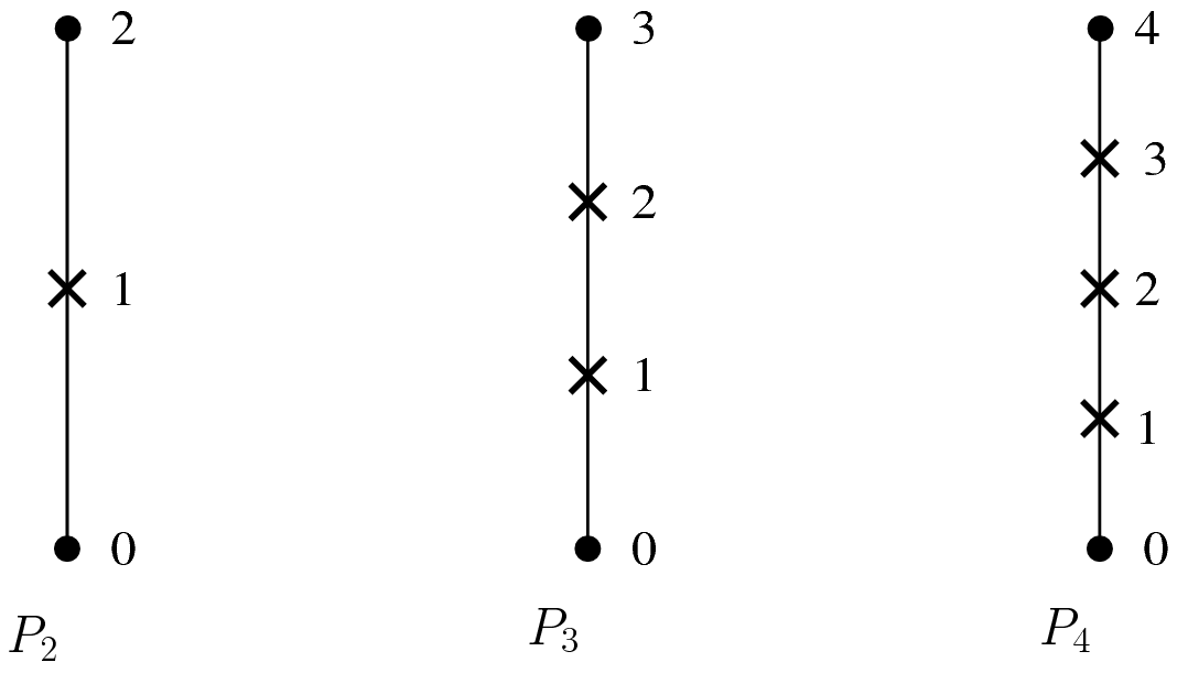
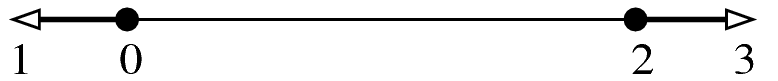
Examples of classical Lagrange elements on a segment
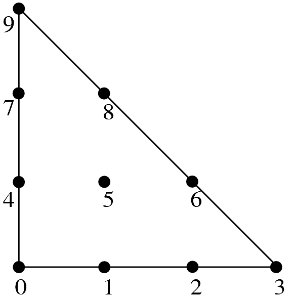
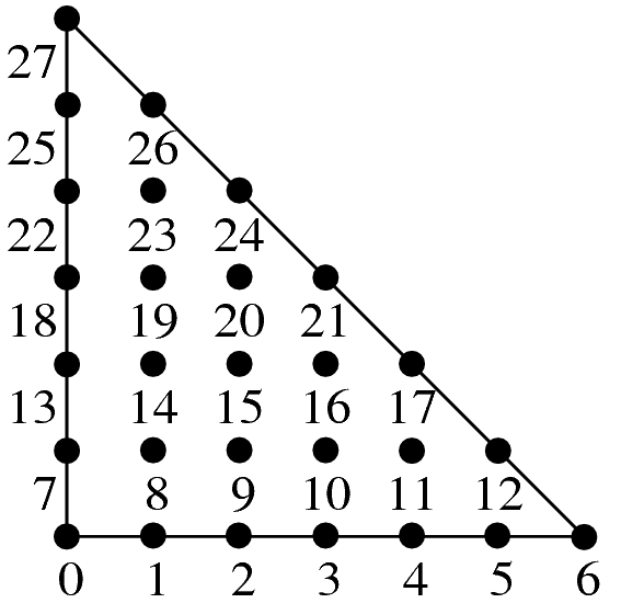
It is possible to define a classical Lagrange element of arbitrary
dimension and arbitrary degree. Each degree of freedom of such an element
corresponds to the value of the function on a corresponding node. The grid of
node is the so-called Lagrange grid. Figures Examples of classical Lagrange elements on a segment.
Examples of classical 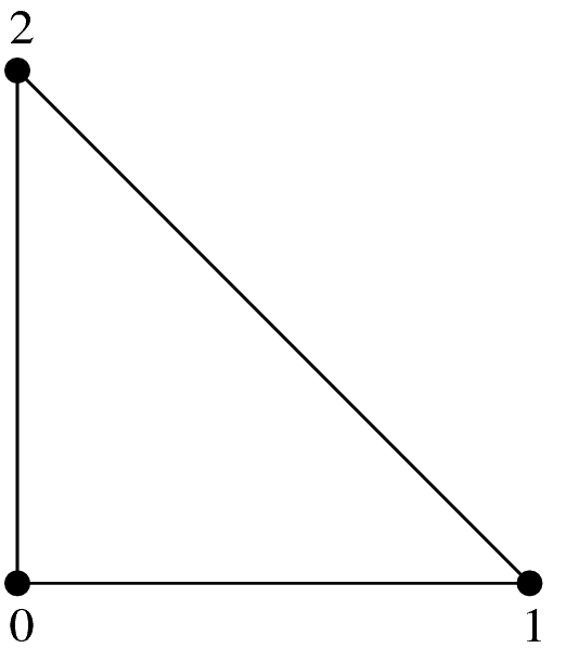
, 3 d.o.f.,
element, 6 d.o.f.,
, 10 d.o.f.,
element, 28 d.o.f.,
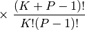
The number of degrees of freedom for a classical Lagrange element of
dimension  and degree
  is
is  . For
instance, in dimension 2
. For
instance, in dimension 2  , this value is
 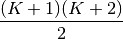 and in dimension 3
  , it is
 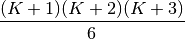 .
.
Examples of classical 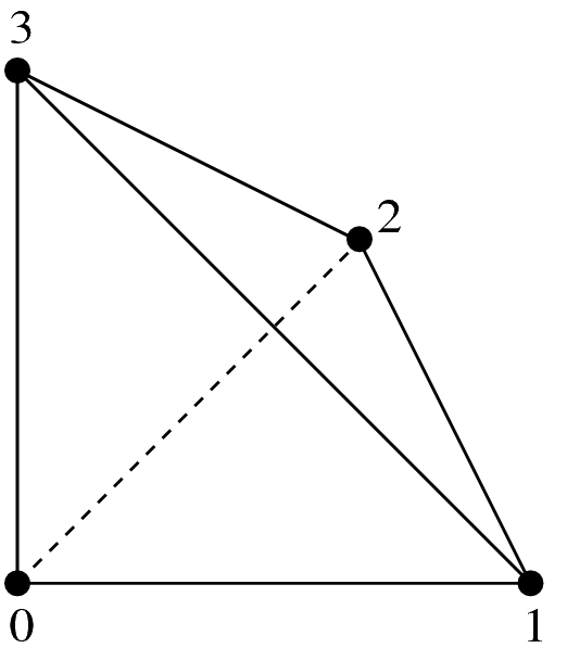
element, 35 d.o.f.,
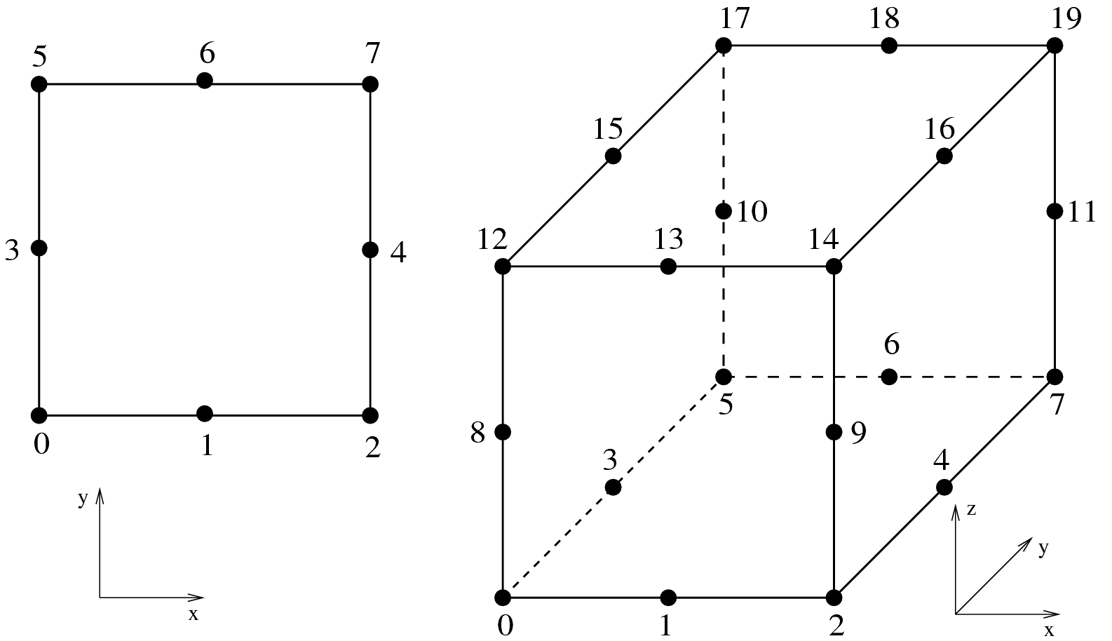
The particular way used in GetFEM++ to numerate the nodes are also shown in figures segment, triangle and tetrahedron. Using another numeration, let

be somme indices such that
Then, the coordinate of a node can be computed as
where  are the vertices of the simplex (for
  the particular choice
 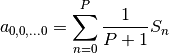 has been chosen). Then each base function, corresponding of each
node
has been chosen). Then each base function, corresponding of each
node  is defined by
where  are the barycentric coordinates, i.e. the polynomials of
degree 1 whose value is
are the barycentric coordinates, i.e. the polynomials of
degree 1 whose value is  on the vertex
  and whose value is
 on other vertices. On the reference element, one has


When between two elements of the same degrees (even with different dimensions),
the d.o.f. of a common face are linked, the element is of class  . This
means that the global polynomial is continuous. If you try to link elements of
different degrees, you will get some trouble with the unlinked d.o.f. This is not
automatically supported by GetFEM++, so you will have to support it (add constraints
on these d.o.f.).
. This
means that the global polynomial is continuous. If you try to link elements of
different degrees, you will get some trouble with the unlinked d.o.f. This is not
automatically supported by GetFEM++, so you will have to support it (add constraints
on these d.o.f.).
For some applications (computation of a gradient for instance) one may not want
the d.o.f. of a common face to be linked. This is why there are two versions of
the classical Lagrange element.
Classical degree dimension d.o.f. number class vector -equivalent
Polynomial No Yes Yes


Discontinuous degree dimension d.o.f. number class vector Polynomial discontinuous No Yes Yes
Even though Lagrange elements are defined for arbitrary degrees, to choose a high degree can be problematic for a large number of applications due to the “noisy” caracteristic of the lagrange basis. These elements are recommended for the basic interpolation but for p.d.e. applications elements with hierarchical basis are preferable (see the corresponding section).
Classical Lagrange elements on other geometries
Classical Lagrange elements on parallelepipeds or prisms are obtained as tensor
product of Lagrange elements on simplices. When two elements are defined, one on a
dimension  and the other in dimension
  , one obtains the base
functions of the tensorial product (on the reference element) as
, one obtains the base
functions of the tensorial product (on the reference element) as

where  and
and  are respectively the base functions
of the first and second element.
are respectively the base functions
of the first and second element.
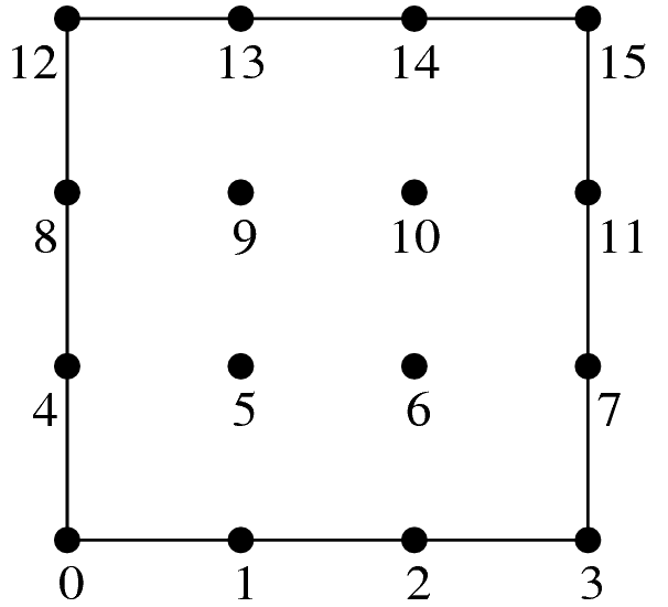
Examples of classical Lagrange elements in dimension 2.
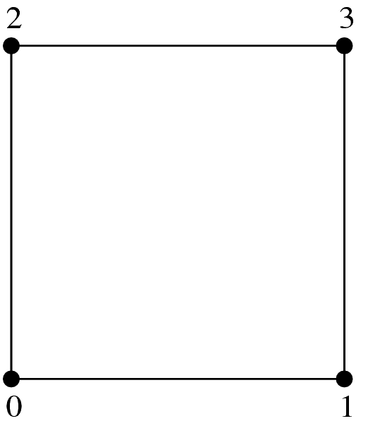
element, 4 d.o.f.,
element, 16 d.o.f.,
The element on a parallelepiped of dimension is obtained as
the tensorial product of classical elements on the segment.
Examples in dimension 2 are shown in figure dimension 2
and in dimension 3 in figure dimension 3.
A prism in dimension  is the direct product of a simplex of dimension
 with a segment. The
  element on this prism is
the tensorial product of the classical element on a simplex of
dimension with the classical element on a segment. For
element on this prism is
the tensorial product of the classical element on a simplex of
dimension with the classical element on a segment. For
 this coincide with a parallelepiped. Examples in dimension
  are shown in figure dimension 3. This is also possible
not to have the same degree on each dimension. An example is shown on figure
dimension 3, prism.
are shown in figure dimension 3. This is also possible
not to have the same degree on each dimension. An example is shown on figure
dimension 3, prism.
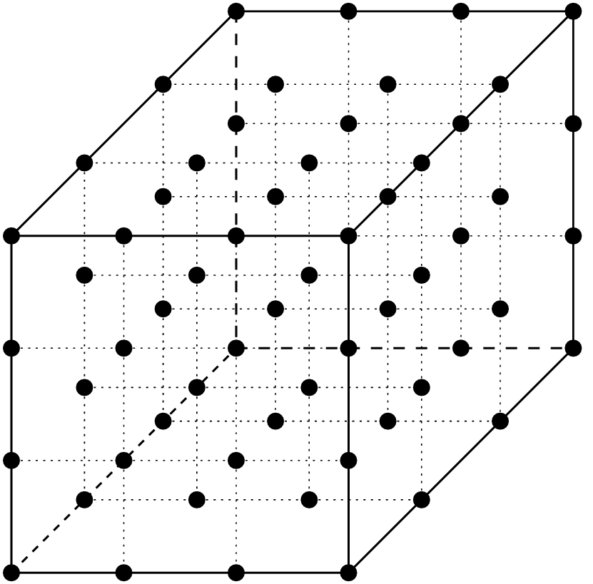
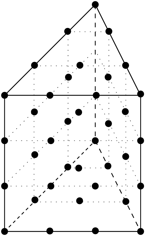
Examples of classical Lagrange elements in dimension 3. 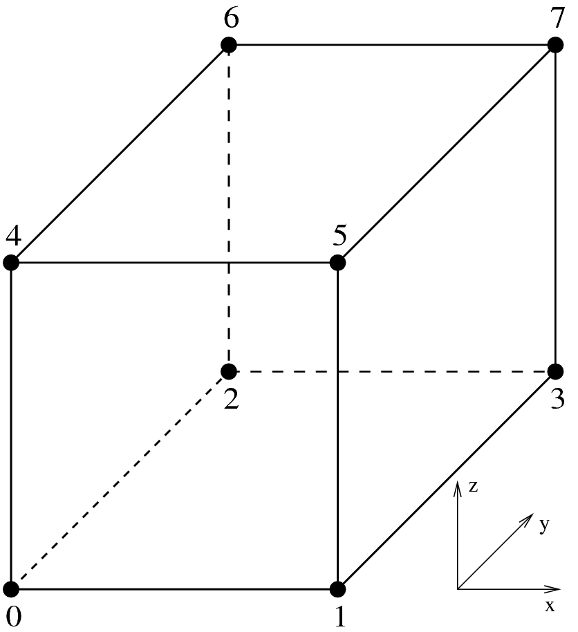
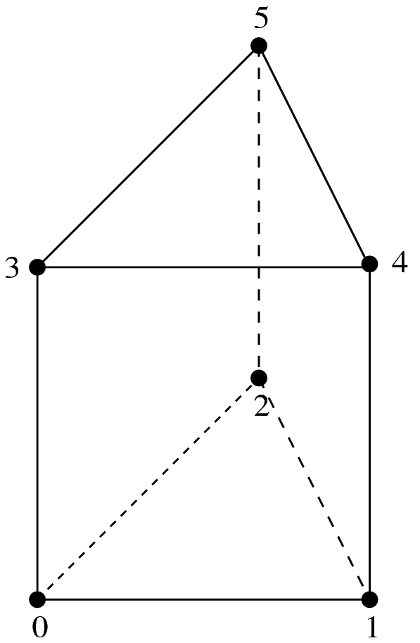
element, 6 d.o.f.,
element, 40 d.o.f.,
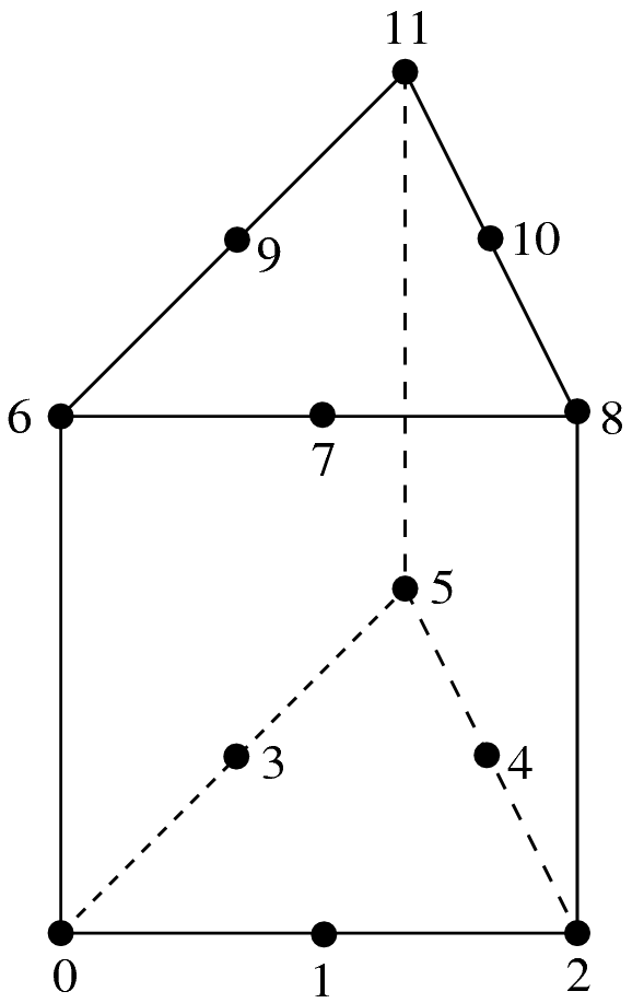
 Lagrange element on a prism, 12 d.o.f.,
. degree dimension d.o.f. number class vector Polynomial ,
No Yes Yes

. degree dimension d.o.f. number class vector Polynomial ,

No Yes Yes

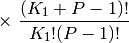
. Lagrange element on prisms "FEM_PRODUCT(FEM_PK(P-1, K1), FEM_PK(1, K2))"
degree dimension d.o.f. number class vector Polynomial ,

No Yes Yes
Incomplete  elements in dimension two and three, 8 or 20 d.o.f.,
Incomplete degree dimension d.o.f. number class vector Polynomial 3 
No Yes Yes


Elements with hierarchical basis
The idea behind hierarchical basis is the description of the solution at different level: a rough level, a more refined level ... In the same discretization some degrees of freedom represent the rough description, some other the more rafined and so on. This corresponds to imbricated spaces of discretization. The hierarchical basis contains a basis of each of these spaces (this is not the case in classical Lagrange elements when the mesh is refined).
Among the advantages, the condition number of rigidity matrices can be greatly improved, it allows local raffinement and a resolution with a multigrid approach.
Hierarchical elements with respect to the degree
Hierarchical element on a segment,
. Classical Lagrange element on simplices but with a hierarchical basis with respect to the degree "FEM_PK_HIERARCHICAL(P,K)"
degree dimension d.o.f. number class vector Polynomial No Yes Yes
. Classical Lagrange element on parallelepipeds but with a hierarchical basis with respect to the degree "FEM_QK_HIERARCHICAL(P,K)"
degree dimension d.o.f. number class vector Polynomial No Yes Yes
. degree dimension d.o.f. number class vector Polynomial No Yes Yes
some particular choices: will be built with the basis of the
, the additional basis of the then the additional basis of the .
will be built with the basis of the , the additional basis
:of the then the additional basis of the (not with the
:basis of the , the additional basis of the then the
:additional basis of the , it is possible to build the latter with
:"FEM_GEN_HIERARCHICAL(a,b)")
Composite elements
The principal interest of the composite elements is to build hierarchical elements. But this tool can also be used to build piecewise polynomial elements.
composite element "FEM_STRUCTURED_COMPOSITE(FEM_PK(2,1), 3)"
Composition of a finite element method on an element with S subdivisions "FEM_STRUCTURED_COMPOSITE(FEM1, S)" degree dimension d.o.f. number class vector Polynomial degree of FEM1 dimension of FEM1 variable variable No If FEM1 is piecewise
It is important to use a corresponding composite integration method.
Hierarchical composite elements

hierarchical composite element "FEM_PK_HIERARCHICAL_COMPOSITE(2,1,3)"
Hierarchical composition of a degree dimension d.o.f. number class vector Polynomial variable No Yes piecewise

Hierarchical composition of a hierarchical degree dimension d.o.f. number class vector Polynomial variable No Yes piecewise
Other constructions are possible thanks to "FEM_GEN_HIERARCHICAL(FEM1, FEM2)" and "FEM_STRUCTURED_COMPOSITE(FEM1, S)".
It is important to use a corresponding composite integration method.
Classical vector elements
Raviart-Thomas of lowest order elements
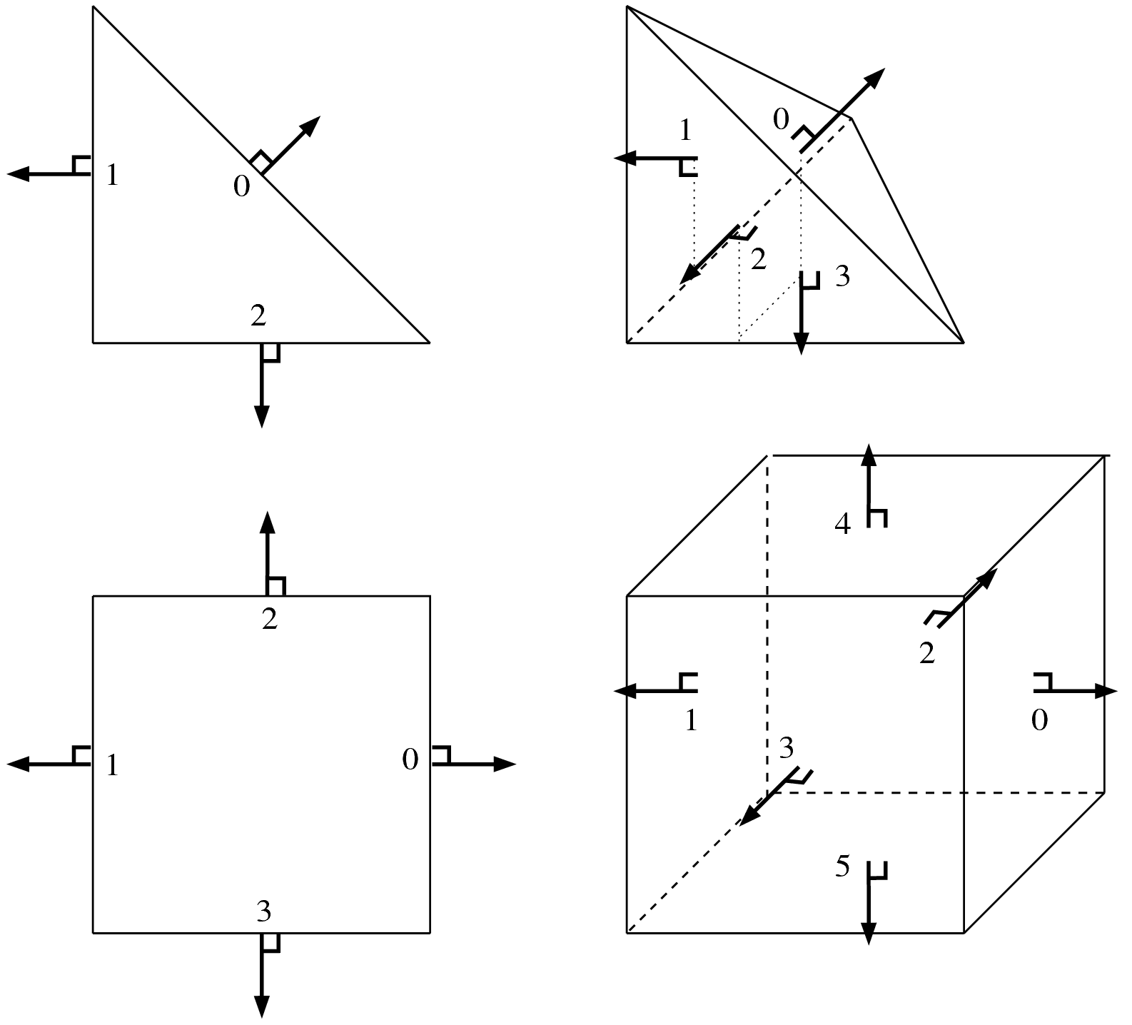
RT0 elements in dimension two and three. (P+1 dof, H(div))
Raviart-Thomas of lowest order element on simplices "FEM_RT0(P)" degree dimension d.o.f. number class vector Polynomial H(div) Yes No Yes


Raviart-Thomas of lowest order element on parallelepipeds (quadrilaterals, hexahedrals) "FEM_RT0Q(P)" degree dimension d.o.f. number class vector Polynomial H(div) Yes No Yes

Nedelec (or Whitney) edge elements
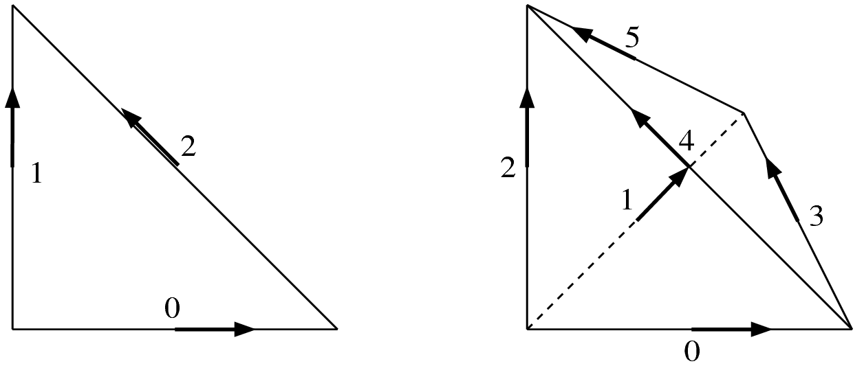
Nedelec edge elements in dimension two and three. (P(P+1)/2 dof, H(rot))
Nedelec (or Whitney) edge element “FEM_NEDELEC(P)”` degree dimension d.o.f. number class vector Polynomial H(rot) Yes No Yes

Specific elements in dimension 1
GaussLobatto element
The 1D GaussLobatto element is similar to the classical
fem on the segment, but the nodes are given by the Gauss-Lobatto-Legendre
quadrature rule of order  . This FEM is known to lead to better
conditioned linear systems, and can be used with the corresponding quadrature to
perform mass-lumping (on segments or parallelepipeds).
. This FEM is known to lead to better
conditioned linear systems, and can be used with the corresponding quadrature to
perform mass-lumping (on segments or parallelepipeds).
The polynomials coefficients have been pre-computed with Maple (they require the
inversion of an ill-conditioned system), hence they are only available for the
following values of :  . Note that for
  and
and  , this is the classical
 and
and  fem.
fem.
GaussLobatto degree dimension d.o.f. number class vector Polynomial No Yes Yes

Hermite element
Hermite element on a segment, 4 d.o.f., 
Base functions on the reference element
This element is close to be -equivalent but it is not. On the real
element the value of the gradient on vertices will be multiplied by the gradient
of the geometric transformation. The matrix  is not equal to identity but
is still diagonal.
is not equal to identity but
is still diagonal.
Hermite element on the segment "FEM_HERMITE(1)" degree dimension d.o.f. number class vector Polynomial No No Yes
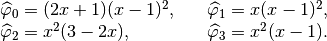
Lagrange element with an additional bubble function
Lagrange element on a segment with additional internal bubble function, 3 d.o.f.,
Lagrange degree dimension d.o.f. number class vector Polynomial No Yes Yes
Specific elements in dimension 2
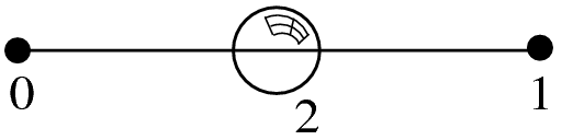
Elements with additional bubble functions
Lagrange element on a triangle with additional internal bubble function 
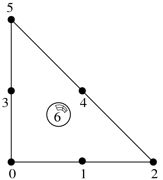
Lagrange degree dimension d.o.f. number class vector Polynomial or
No Yes Yes

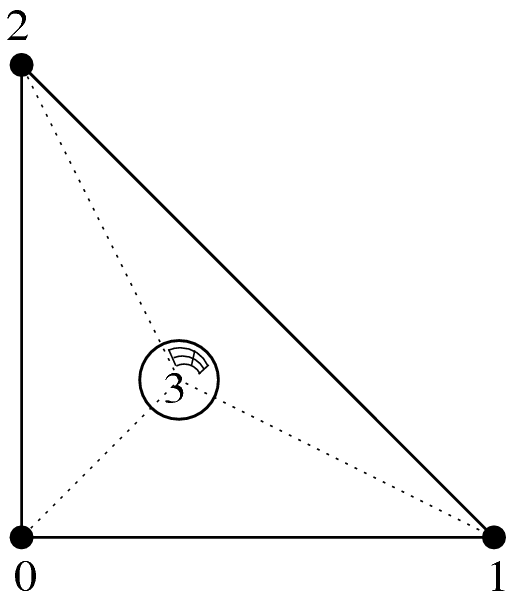
Lagrange element on a triangle with additional internal piecewise linear bubble function
Lagrange degree dimension d.o.f. number class vector Polynomial No Yes Piecewise
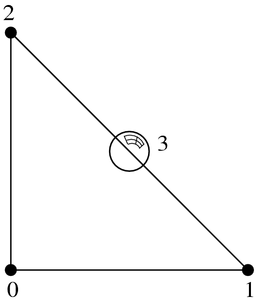
Lagrange element on a triangle with additional bubble function on face 0, 4 d.o.f.,
Lagrange degree dimension d.o.f. number class vector Polynomial No Yes Yes
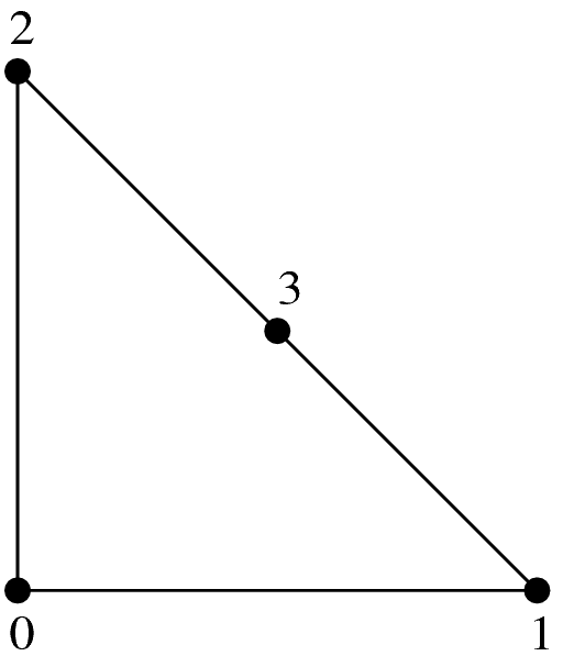
Lagrange element on a triangle with additional d.o.f on face 0, 4 d.o.f.,
. degree dimension d.o.f. number class vector Polynomial No Yes Yes
Non-conforming element
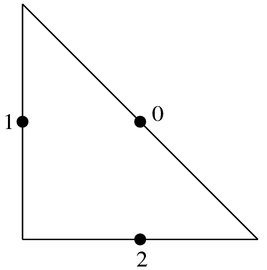
non-conforming element on a triangle, 3 d.o.f., discontinuous
. degree dimension d.o.f. number class vector Polynomial No Yes Yes
Hermite element
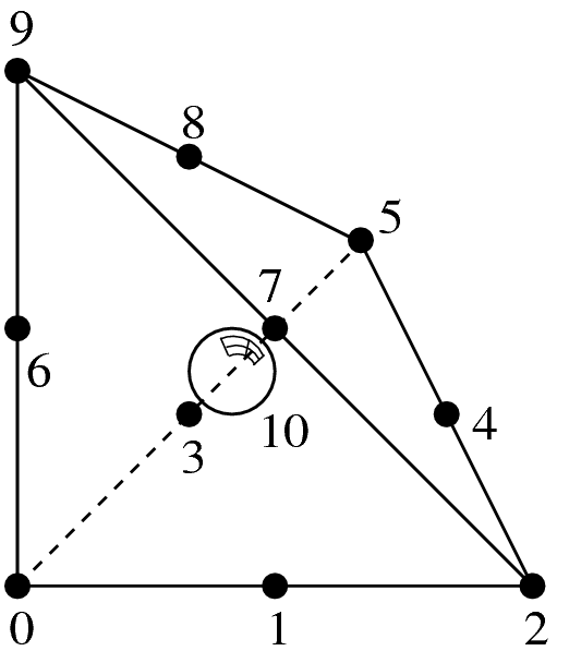
Hermite element on a triangle, , 10 d.o.f.,
Base functions on the reference element:
This element is not -equivalent (The matrix is not equal to
identity). On the real element linear combinations of  and
and
 are used to match the gradient on the corresponding vertex.
Idem for the two couples
are used to match the gradient on the corresponding vertex.
Idem for the two couples  ,
,  and
and
 ,
,  for the two other vertices.
Hermite element on a triangle "FEM_HERMITE(2)" degree dimension d.o.f. number class vector Polynomial No No Yes

Morley element
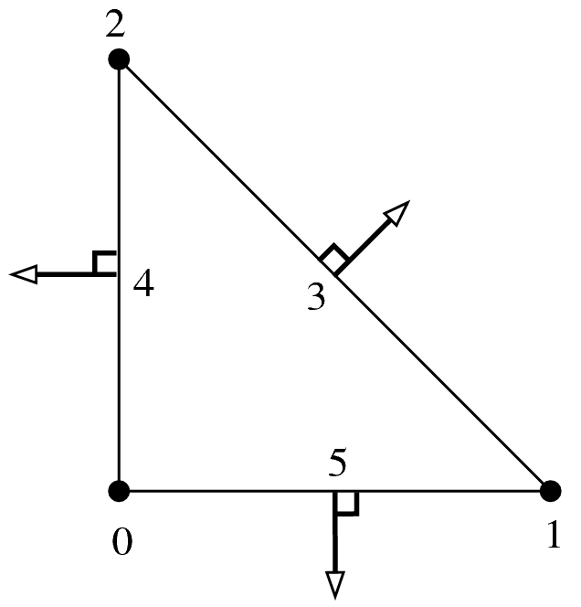
triangle Morley element, , 6 d.o.f.,
This element is not -equivalent (The matrix is not equal to
identity). In particular, it can be used for non-conforming discretization of
fourth order problems, despite the fact that it is not  .
.
Morley element on a triangle "FEM_MORLEY" degree dimension d.o.f. number class vector Polynomial discontinuous No No Yes

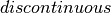
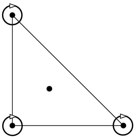
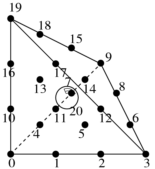
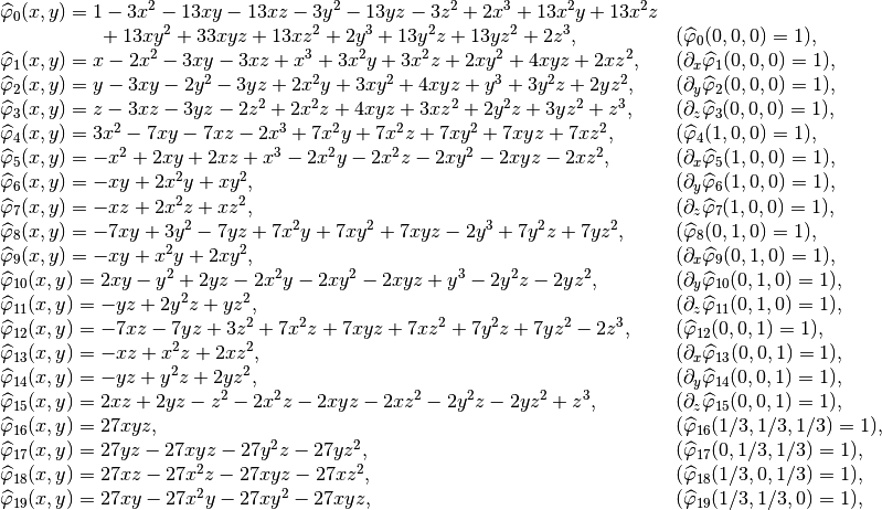
Argyris element
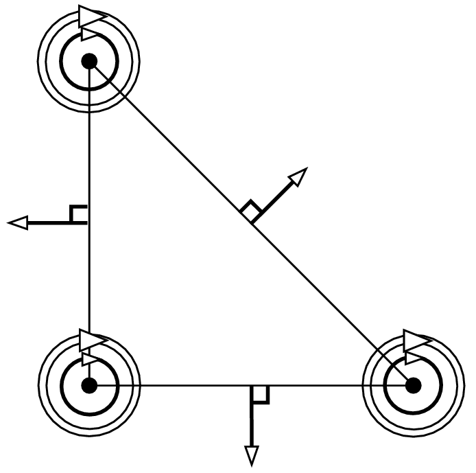
Argyris element,  , 21 d.o.f.,
The base functions on the reference element are:
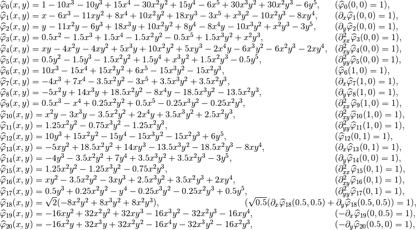
This element is not -equivalent (The matrix is not equal to
identity). On the real element linear combinations of the transformed base
functions  are used to match the gradient, the second
derivatives and the normal derivatives on the faces. Note that the use of the
matrix allows to define Argyris element even with nonlinear geometric
transformations (for instance to treat curved boundaries).
are used to match the gradient, the second
derivatives and the normal derivatives on the faces. Note that the use of the
matrix allows to define Argyris element even with nonlinear geometric
transformations (for instance to treat curved boundaries).
Argyris element on a triangle "FEM_ARGYRIS" degree dimension d.o.f. number class vector Polynomial No No Yes

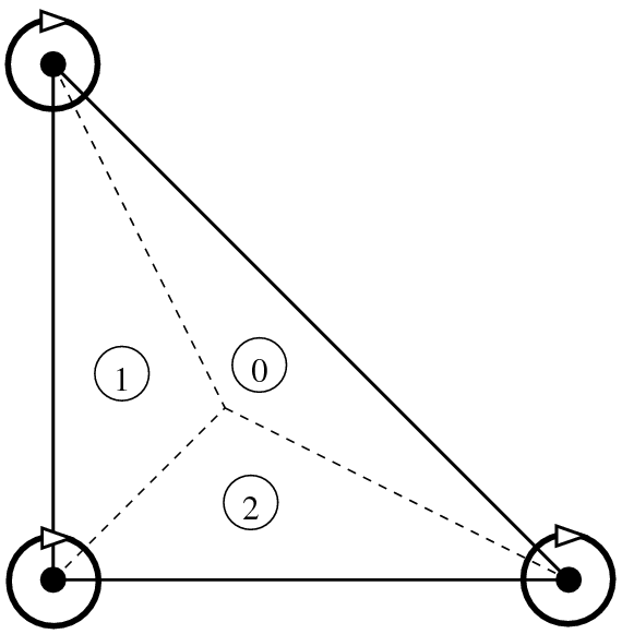
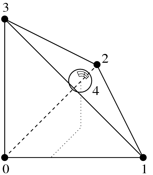
Hsieh-Clough-Tocher element
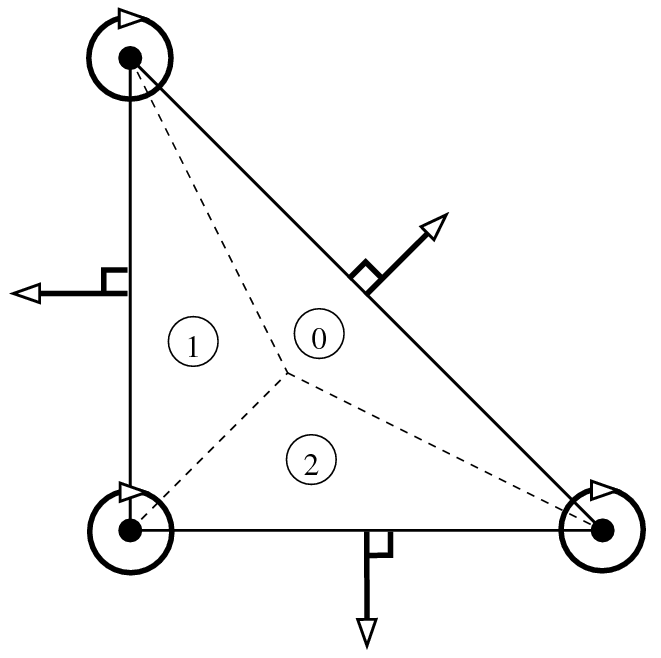
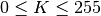
Hsieh-Clough-Tocher (HCT) element, , 12 d.o.f.,
This element is not -equivalent. This is a composite element.
Polynomial of degree 3 on each of the three sub-triangles (see figure
Hsieh-Clough-Tocher (HCT) element, , 12 d.o.f., and [ciarlet1978]). It is strongly advised to use a
"IM_HCT_COMPOSITE" integration method with this finite element. The numeration
of the dof is the following: 0, 3 and 6 for the lagrange dof on the first second
and third vertex respectively; 1, 4, 7 for the derivative with respects to the
first variable; 2, 5, 8 for the derivative with respects to the second variable
and 9, 10, 11 for the normal derivatives on face 0, 1, 2 respectively.
HCT element on a triangle "FEM_HCT_TRIANGLE" degree dimension d.o.f. number class vector Polynomial No No piecewise

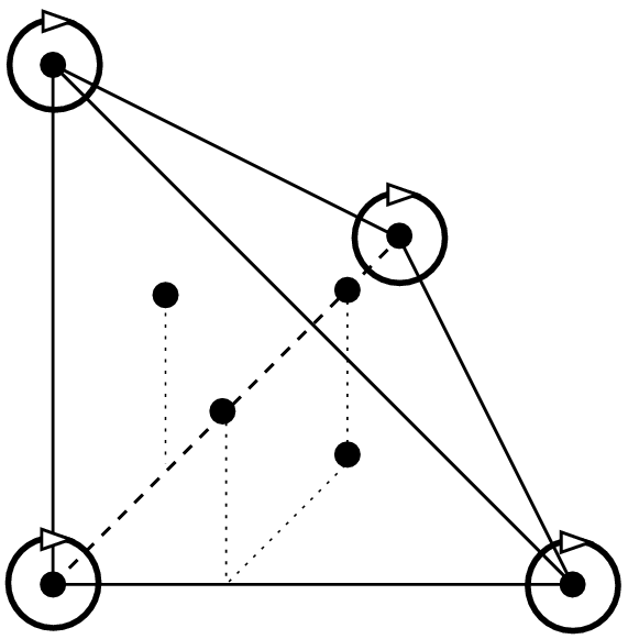
Reduced Hsieh-Clough-Tocher (reduced HCT) element, , 9 d.o.f.,
This element exists also in its reduced form, where the normal derivatives are assumed to be polynomial of degree one on each edge (see figure Reduced Hsieh-Clough-Tocher (reduced HCT) element, , 9 d.o.f., )
Reduced HCT element on a triangle "FEM_REDUCED_HCT_TRIANGLE" degree dimension d.o.f. number class vector Polynomial No No piecewise

A composite element on quadrilaterals
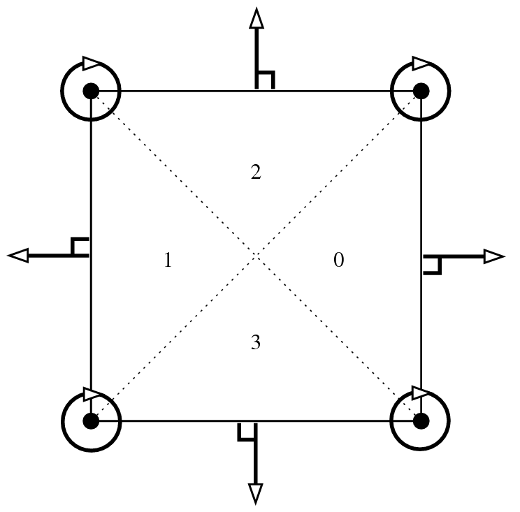
Composite element on quadrilaterals, piecewise , 16 d.o.f.,
This element is not -equivalent. This is a composite element.
Polynomial of degree 3 on each of the four sub-triangles (see figure
Composite element on quadrilaterals, piecewise , 16 d.o.f., ). At least on the reference element it corresponds to the
Fraeijs de Veubeke-Sander element (see [ciarlet1978]). It is strongly advised
to use a "IM_QUADC1_COMPOSITE" integration method with this finite element.
. degree dimension d.o.f. number class vector Polynomial No No piecewise

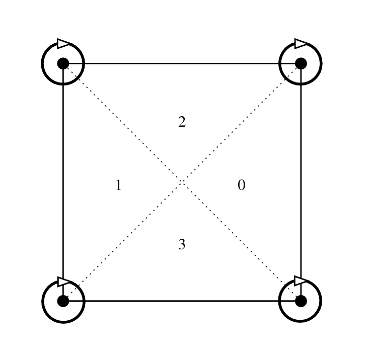
Reduced composite element on quadrilaterals, piecewise , 12 d.o.f.,
This element exists also in its reduced form, where the normal derivatives are assumed to be polynomial of degree one on each edge (see figure Reduced composite element on quadrilaterals, piecewise , 12 d.o.f., )
Reduced degree dimension d.o.f. number class vector Polynomial No No piecewise
Specific elements in dimension 3
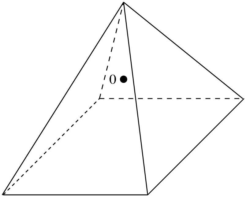
Lagrange elements on 3D pyramid
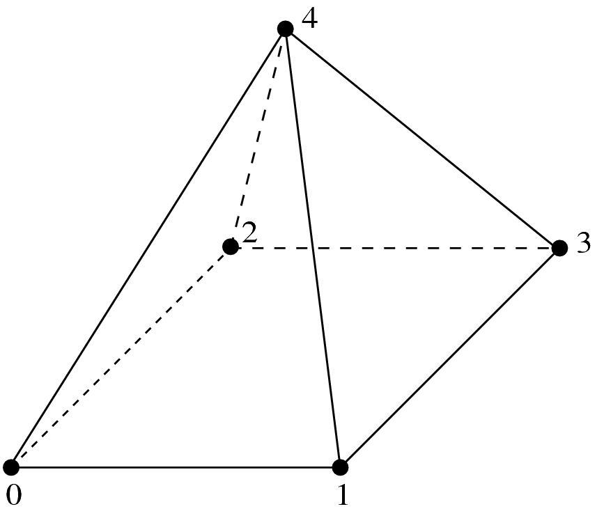
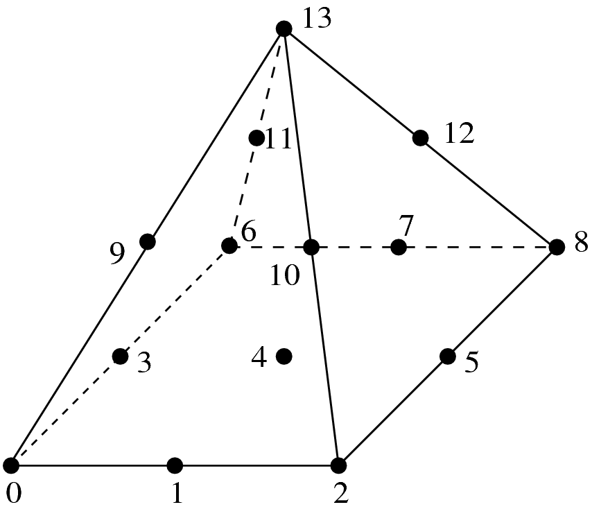
GetFEM++ proposes some Lagrange pyramidal elements of degree 0, 1 and two based on [GR-GH1999] and [BE-CO-DU2010]. See these references for more details. The proposed element can be raccorded to standard or Lagrange fem on the triangular faces and to a standard or Lagrange fem on the quatrilateral face.
|
|
|
| Degree 0 pyramidal element with 1 dof | Degree 1 pyramidal element with 5 dof | Degree 2 pyramidal element with 14 dof |
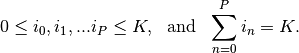
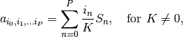
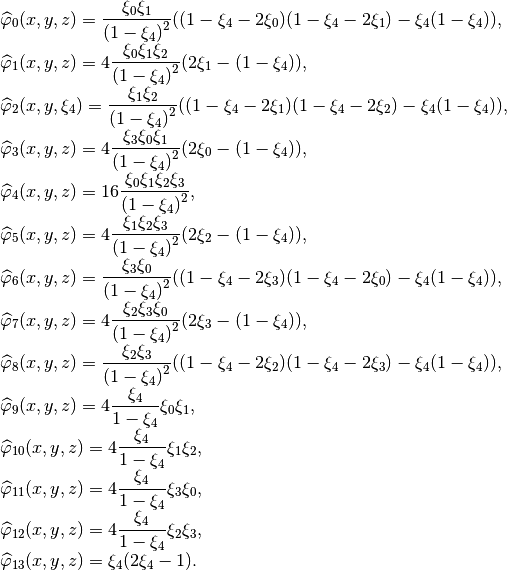
The associated geometric transformations are "GT_PYRAMID(K)" for K = 1 or 2. The associated integration methods "IM_PYRAMID(im)" where im is an integration method on a hexahedron (or alternatively "IM_PYRAMID_COMPOSITE(im)" where im is an integration method on a tetrahedron, but it is theoretically less accurate) The shape functions are not polynomial ones but rational fractions. For the first degree the shape functions read:

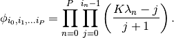
For the second degree, setting

the shape functions read:
| degree | dimension | d.o.f. number | class | vector | -equivalent |
Polynomial |
|---|---|---|---|---|---|---|
|
|
|
discontinuous | No  |
Yes | No |
|
|
 |
|
No |
Yes | No |
 |
|
 |
|
No |
Yes | No |
| degree | dimension | d.o.f. number | class | vector | -equivalent |
Polynomial |
|---|---|---|---|---|---|---|
|
|
|
discontinuous | No |
Yes | No |
|
|
|
discontinuous | No |
Yes | No |
|
|
|
discontinuous | No |
Yes | No |
Elements with additional bubble functions
Lagrange element on a tetrahedron with additional internal bubble function 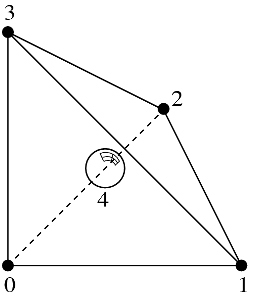
degree dimension d.o.f. number class vector Polynomial or
No Yes Yes
Lagrange element on a tetrahedron with additional bubble function on face 0, 5 d.o.f.,
Lagrange degree dimension d.o.f. number class vector Polynomial No Yes Yes
Hermite element
Hermite element on a tetrahedron, , 20 d.o.f.,
Base functions on the reference element:
This element is not -equivalent (The matrix is not equal to
identity). On the real element linear combinations of  ,
,
 and
and  are used to match the gradient on
the corresponding vertex. Idem on the other vertices.
are used to match the gradient on
the corresponding vertex. Idem on the other vertices.
Hermite element on a tetrahedron "FEM_HERMITE(3)" degree dimension d.o.f. number class vector Polynomial No No Yes

![]()
Table Of Contents
- Appendix A. Finite element method list
Previous topic
ALE Support for object having a large rigid body motion
Next topic
Appendix B. Cubature method list
Download
Main documentations
- GetFEM++ User documentation
- Python Interface
- Matlab Interface
- Scilab Interface
- Gmm++
- GetFEM++ project