Appendix A. Some basic computations between reference and real elements
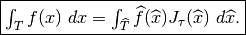
Volume integral
One has

Denoting  the jacobian

one finally has
When  , the expression of the jacobian reduces to
 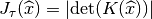 .
.
Surface integral
With  a part of the boundary of
  a real element and
 the corresponding boundary on the reference element
  ,
one has
,
one has
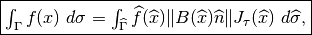
where  is the unit normal to on . In a same
way
is the unit normal to on . In a same
way

For  the unit normal to on .
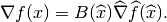
Second derivative computation
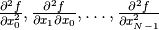
Denoting
![\nabla^2 f =
\left[\frac{\partial^2 f}{\partial x_i \partial x_j}\right]_{ij},](../_images/math/922650db95a714a428af3c384a4e359d258de17e.png)
the  matrix and
the  matrix, then

and thus

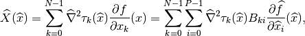
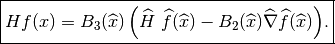
In order to have uniform methods for the computation of elementary matrices, the
Hessian is computed as a column vector  whose components are
 . Then, with
 the
the  matrix defined as
![\left[B_2(\widehat{x})\right]_{ij} =
\sum_{k = 0}^{N-1}
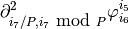
\frac{\partial^2 \tau_k(\widehat{x})}{\partial \widehat{x}_{i / P} \partial \widehat{x}_{i\mbox{ mod }P}}
B_{kj}(\widehat{x}),](../_images/math/af0dc2d4ddff4d7e7c23ea66da969f7cd3547afb.png)
and  the
the  matrix defined as
![\left[B_3(\widehat{x})\right]_{ij} =
B_{i / N, j / P}(\widehat{x}) B_{i\mbox{ mod }N, j\mbox{ mod }P}(\widehat{x}),](../_images/math/a154bfb20b9d7666d4d1ac1dc4f0ea257870ff0d.png)
one has
Example of elementary matrix
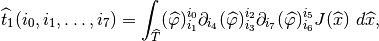
Assume one needs to compute the elementary “matrix”:
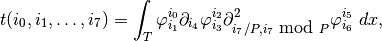
The computations to be made on the reference elements are

and
Those two tensor can be computed once on the whole reference element if the
geometric transformation is linear (because  is constant). If the
geometric transformation is non-linear, what has to be stored is the value on
each integration point. To compute the integral on the real element a certain
number of reductions have to be made:
is constant). If the
geometric transformation is non-linear, what has to be stored is the value on
each integration point. To compute the integral on the real element a certain
number of reductions have to be made:
- Concerning the first term (
 ) nothing.
 - Concerning the second term (
 ) a
reduction with respect to
) a
reduction with respect to  with the matrix
  .
. - Concerning the third term (
 )` a reduction of
  with respect to
  with the matrix and a reduction of
  with respect also
to with the matrix
with respect also
to with the matrix 
The reductions are to be made on each integration point if the geometric transformation is non-linear. Once those reductions are done, an addition of all the tensor resulting of those reductions is made (with a factor equal to the load of each integration point if the geometric transformation is non-linear).
If the finite element is non- -equivalent, a supplementary reduction of the
resulting tensor with the matrix
-equivalent, a supplementary reduction of the
resulting tensor with the matrix  has to be made.
![]()
Table Of Contents
Previous topic
Interface with scripts languages (Python, Scilab and Matlab)
Next topic
Download
Main documentations
- GetFEM++ User documentation
- Python Interface
- Matlab Interface
- Scilab Interface
- Gmm++
- GetFEM++ project